


 Reviewed by
Price elasticity of demand (PED) measures how a change in price affects the quantity of a product consumers are willing to buy. It's one of the most important concepts in microeconomics, helping businesses and economists predict how pricing changes will impact demand, total revenue, and profitability.
Below is a free price elasticity of demand calculator and a breakdown of PED types, formulas, and real-world examples. I'll explain how to use the midpoint method to calculate elasticity, interpret whether demand is elastic, inelastic, or unitary, and apply these insights to build stronger pricing strategies.
Price Elasticity of Demand Calculator
This easy-to-use price elasticity calculator computes PED instantly. Enter your initial and new prices and quantities, and it will show your elasticity coefficient along with whether demand is elastic, inelastic, or unitary. This can help you understand how sensitive your customers are to price changes so you can make smarter pricing decisions.
The PED calculator is useful for:
Business owners reviewing pricing strategies
Students studying microeconomics
Pricing analysts modeling revenue impact
What Is Price Elasticity of Demand?
Price elasticity of demand measures how much the quantity demanded of a product changes in response to a change in its price. It helps explain consumer behavior: When prices go up or down, how likely are customers to adjust how much they buy?
Economists and business owners use PED to forecast revenue, optimize pricing, and understand shifts in the demand curve. In microeconomics, it's a foundational concept for analyzing how pricing decisions impact total revenue.
The basic idea is simple: if a small price change leads to a big change in quantity demanded, the product is elastic. If quantity barely changes, the product is inelastic. PED is typically expressed as an absolute value (ignoring the negative sign), so a result of 2.0 means demand is highly elastic regardless of direction.
The basic elasticity formula is:
Price Elasticity of Demand (PED) = (% Change in Quantity Demanded) ÷ (% Change in Price)
This is the formula our calculator above uses.
How Price Elasticity of Demand Works
There are two common approaches to calculating PED: the basic percentage change method and the midpoint method. Both use the same core elasticity formula, but the midpoint method is more accurate when working with larger price changes.
Basic Percentage Change Method
This divides the percent change in quantity demanded by the percent change in price. Here's an example:
A retailer sells 500 units of a product at $20 each. After raising the price to $25, sales drop to 400 units.
Percent change in quantity:
(400 − 500) ÷ 500 = −20%Percent change in price:
($25 − $20) ÷ $20 = 25%PED =
−20% ÷ 25% = −0.8
The absolute value is 0.8, which means demand is inelastic. The price increase didn't cause a proportional drop in quantity demanded.
The Midpoint Formula
The midpoint method (also called the arc elasticity method) uses the average of the initial and final values as the base for calculating percentage changes. This avoids the problem where calculating elasticity from point A to point B gives a different result than calculating from B to A.
The midpoint formula is:
PED =
New Qty − Initial Qty
(New Qty + Initial Qty) ÷ 2New Price − Initial Price
(New Price + Initial Price) ÷ 2Here's a worked example using the midpoint method:
Suppose a business raises its price from $10 (initial price) to $12 (new price), and the quantity demanded drops from 100 units (initial quantity) to 80 units (new quantity). The steps would be:
Calculate the percentage change in quantity:
(80 − 100) ÷ ((80 + 100) ÷ 2) = −20 ÷ 90 = −22.2%Calculate the percentage change in price:
($12 − $10) ÷ (($12 + $10) ÷ 2) = $2 ÷ $11 = 18.2%Divide the quantity change by the price change:
PED = −22.2% ÷ 18.2% = −1.22
The absolute value of the elasticity coefficient is 1.22, which means demand is elastic. A 1% increase in the average price leads to roughly a 1.22% decrease in quantity demanded. For this product, price increases would likely reduce total revenue.
Types of Elasticity: What the Results Mean
Once you calculate the price elasticity of demand, the elasticity coefficient tells you how sensitive customers are to price changes and what effect those changes have on total revenue.
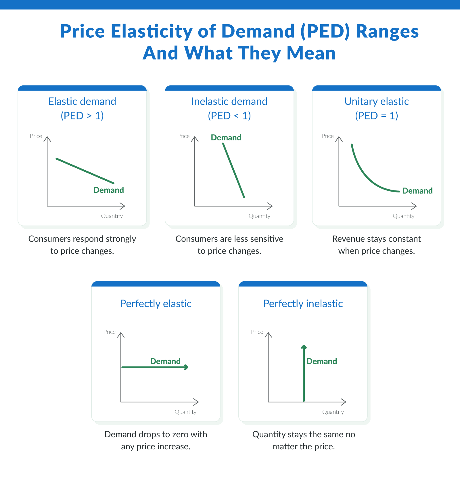
Elastic demand (PED > 1)
Consumers respond strongly to price changes. A small price increase can cause a large drop in quantity demanded, potentially decreasing total revenue. Examples: luxury items, non-essential electronics, trendy fashion products.
Inelastic demand (PED < 1)
Consumers are less sensitive to price changes. Quantity demanded changes only slightly, so raising prices may increase total revenue. Examples: gasoline, prescription drugs, basic food staples.
Unitary elastic (PED = 1)
Price and quantity move in exact proportion, so total revenue stays the same regardless of a price change. Examples: products near a balanced demand curve, like certain mid-range household items.
Perfectly elastic (PED = infinity)
Any price increase causes the quantity demanded to drop to zero. Consumers will only buy at one exact price. Examples: commodities in perfectly competitive markets where identical substitutes are available at the market price.
Perfectly inelastic (PED = 0)
Quantity demanded doesn't change at all, regardless of price. Consumers need the product no matter the cost. Examples: life-saving medications with no alternatives, like insulin for diabetic patients.
Knowing where your product falls on the elasticity scale helps you decide whether a price increase or price decrease is likely to grow or shrink revenue.
What Affects Price Elasticity?
Several things influence how elastic or inelastic a product's demand will be. Understanding them can help you anticipate customer behavior when making pricing decisions:
Availability of substitutes. The more alternatives available, the more elastic the demand. Customers will switch if your price rises.
Necessity vs. luxury. Essential items (like medication or utilities) are generally inelastic. Luxury goods tend to be more elastic.
Time period. Demand often becomes more elastic over time as customers adjust or find alternatives.
Price point. Items with higher prices usually face more elastic demand since price changes have a bigger impact on the total amount spent.
Product category. Some categories consistently show stable demand regardless of price shifts, especially when products are unique or habit-forming. Analyzing the demand function for your product category can reveal where optimization opportunities exist.
These insights are key for economists, marketers, and business owners shaping demand curve models and pricing strategies.
Related Types of Elasticity
Price elasticity of demand isn't the only elasticity measure that matters for pricing and business strategy. Three related concepts help round out the picture:
Cross-price elasticity
Measures how the quantity demanded of one product changes when the price of a related product changes. A positive value means the products are substitutes (one brand of coffee vs. another). A negative value means they're complements (printers and ink cartridges). This metric helps you understand how competitor pricing affects your sales.
Income elasticity
Measures how quantity demanded changes as consumer income changes. Luxury goods tend to have high income elasticity (demand rises sharply when people earn more). Necessities have low income elasticity since people buy them regardless of income.
Price elasticity of supply
Measures how much the quantity supplied changes in response to a price change. While PED focuses on the buyer's side, price elasticity of supply looks at the seller's ability to adjust production. Products that are easy to manufacture quickly tend to have elastic supply.
Using PED To Improve Pricing Strategy
Understanding price elasticity of demand can help business owners make smarter pricing decisions, boost total revenue, and respond quickly to shifts in customer behavior. Whether you're weighing price increases or price decreases, elasticity insights give you a roadmap for protecting your margins and growing your business.
Here are practical ways to apply PED to real-world pricing strategies:

Raise prices carefully on inelastic products to maximize revenue
When demand changes very little after a price increase, you can grow total revenue without losing many sales. Look at the initial quantity sold, forecast the final quantity after the change, and estimate the percentage change to guide your decision.

Lower prices on elastic products to drive higher sales volume
When customers respond strongly to lower prices, a small price decrease can lead to a large increase in units sold, helping you achieve a revenue increase overall.

Maintain stable pricing on unit elastic products
If the percent change in quantity matches the percent change in price, total revenue stays about the same. In these cases, focusing on operational optimization may have a bigger impact than adjusting prices.

Model different pricing scenarios
By comparing your initial price, final price, initial quantity, and expected final quantity, you can predict how different price points will impact demand changes and total revenue.

Test and adjust based on actual results
PED gives you a strong starting point, but real-world data matters. Watch how customers respond after a price adjustment and refine your strategy accordingly. If price rises lead to steeper-than-expected drops in sales, your product may be more elastic than you estimated.
Building pricing strategies with elasticity in mind helps you move from guesswork to data-driven decisions and positions your business for smarter, more sustainable business growth.
Understand Elasticity for Smarter Pricing Decisions
Price elasticity of demand is a practical tool for small businesses looking to make confident, informed pricing moves. Whether you're launching a new product, responding to competitors, or planning a price adjustment, elasticity insights help you predict customer behavior and protect total revenue.
Bookmark this quick guide and the price elasticity of demand calculator for future use. Having a fast way to estimate how demand curves respond will help you make better pricing decisions and stay ahead of market changes. Economists, pricing teams, and business owners rely on PED models to turn small changes into major advantages.
Ready to put your insights into action and fund your next business move? Apply with Clarify Capital and get matched with fast, flexible financing options built for small businesses.
FAQ
People often ask questions like these when we're discussing price elasticity of demand.
What Does a Price Elasticity of Demand of 1.5 Mean?
A PED of 1.5 means demand is elastic. For every 1% increase in price, the quantity demanded drops by 1.5%. Since the percentage change in quantity is larger than the percentage change in price, raising prices would likely decrease total revenue.
Is Inelastic Demand Less Than 1?
Yes. Inelastic demand has an absolute value less than 1 (but greater than 0). This means quantity demanded changes less than proportionally to price. For example, a PED of 0.4 means a 1% price increase only reduces quantity demanded by 0.4%.
What Is the Difference Between Price Elasticity of Demand and Price Elasticity of Supply?
Price elasticity of demand measures how buyers respond to price changes (changes in quantity demanded). Price elasticity of supply measures how sellers respond to price changes (changes in quantity supplied). Both use similar formulas, but PED focuses on consumer behavior while supply elasticity focuses on production capacity and manufacturer response times.
What Are the Limitations of Using Price Elasticity of Demand?
PED assumes all other factors stay constant, which rarely happens in real markets. It also captures a snapshot in time and may not reflect long-term demand shifts. External factors like seasonality, competitor actions, and macroeconomic changes can all influence the relationship between price and quantity demanded in ways the formula doesn't account for.

Michael Baynes
Co-founder, Clarify
Michael has over 15 years of experience in the business finance industry working directly with entrepreneurs. He co-founded Clarify Capital with the mission to cut through the noise in the finance industry by providing fast funding and clear answers. He holds dual degrees in Accounting and Finance from the Kelley School of Business at Indiana University. More about the Clarify team →
Related Posts